Price-Response Asymmetry And Spatial Differentiation In Local Retail Gasoline Markets
| This document is available in two formats: this web page (for browsing content) and PDF (comparable to original document formatting). To view the PDF you will need Acrobat Reader, which may be downloaded from the Adobe site. |
| ECONOMIC ANALYSIS GROUP
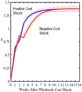
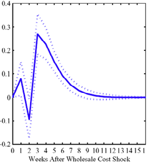
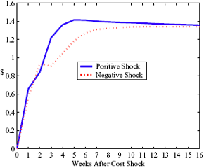
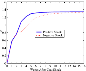
EAG Discussion Papers are the primary vehicle used to disseminate research from economists in the Economic Analysis Group (EAG) of the Antitrust Division. These papers are intended to inform interested individuals and institutions of EAG's research program and to stimulate comment and criticism on economic issues related to antitrust policy and regulation. The analysis and conclusions expressed herein are solely those of the authors and do not represent the views of the United States Department of Justice. Information on the EAG research program and discussion paper series may be obtained from Russell Pittman, Director of Economic Research, Economic Analysis Group, Antitrust Division, U.S. Department of Justice, BICN 10-000, Washington, DC 20530, or by e-mail at russell.pittman@usdoj.gov. Comments on specific papers may be addressed directly to the authors at the same mailing address or at their e-mail address. Recent EAG Discussion Paper titles are listed at the end of this paper. To obtain a complete list of titles or to request single copies of individual papers, please write to Janet Ficco at the above mailing address or at janet.ficco@usdoj.gov or call (202) 307-3779. Beginning with papers issued in 1999, copies of individual papers are also available from the Social Science Research Network at www.ssrn.com. Abstract This study explores the possibility that local market power influences the observed asymmetric relationship between changes in wholesale gasoline costs and changes in retail gasoline prices. I exploit an original data set of weekly gas station prices in Southern California from September 2002 to May 2003, and take advantage of detailed station and local market level characteristics to determine the extent to which spatial differentiation influences price response asymmetry. I find that brand identity, proximity to rival stations, bundling and advertising, operation type, and local market features and demographics each influence a station's predicted price-response asymmetry. 1 Introduction The pricing dynamics of retail gasoline have resurfaced as an important policy issue in the last few years. Of particular concern is the observed phenomenon that prices respond asymmetrically to cost shocksprices rise at a much faster rate with cost increases than they do with cost declines. Research into the possible sources of this asymmetry remains an ongoing concern. In this study, I investigate the extent to which local market power may contribute to price asymmetry. Past studies have found only limited support for the hypothesis that market power influences pricing dynamics. Part of the difficulty is that for the retail sector in the gasoline industry, market power occurs at the local or station level through geographic and other forms of spatial differentiation. However, most gasoline pricing studies employ publicly available aggregate data on prices, usually at a regional level. The few emerging studies that take advantage of station-level data are generally cross-sections, which are unable by definition to describe the types of pricing dynamics discussed here. I overcome these data complications by collecting a station-level data set of weekly retail gasoline prices from September 2002 to May 2003, which I use to examine how station-specific characteristics such as location relative to competitors, consumers, and major infrastructures are potential sources of market power, and thus how they contribute to pricing asymmetry at a micro level. In this paper, I establish that price-response asymmetry is a dominant feature in my data set, and explore the possibility that certain station-level features such as brand identity and other site- and local-market characteristics exhibit varying degrees of asymmetry consistent with a positive local market power effect. I assume that each station has its own response to current and lagged cost and price changes, that these effects depend explicitly on its site- and local-market specific characteristics, and that these effects are themselves correlated with each other as a function of the geographic distance between stations. Specifically, I find that, aggregated across all stations, three weeks after a singleton wholesale cost increase of 100¢, retail prices are predicted to rise an estimated 110¢; but when costs fall by 100¢, retail prices only fall by 83¢. This 27¢ difference, which I define as the price-response asymmetry, declines gradually toward zero after the third week until retail prices settle at their estimated long-run response. I also find that brand identity contributes measurably to asymmetry: three weeks after a wholesale cost shock, the asymmetry for the highest-priced brands is estimated at 34¢, while for unbranded stations the difference in responses is estimated at only 14¢. Regarding the benefit of geographic isolation, I find that stations with no rivals in immediate proximity exhibit an asymmetry after the third week that is approximately 7¢ greater than if these same stations had a neighbor immediately nearby. I also find that after the third week following a cost shock, the difference in asymmetry for stations with greater versus lesser ease-of-access is approximately 20¢, diminishing slowly toward zero afterward. Similar results, though different in magnitude, are attributed to stations with a convenience store and to stations with relatively more pumps on their lot. Lastly, I find that more competitive local markets have a lower price-response asymmetry by 10¢ at the third week after a cost shock, while a one standard deviation increase in the local market population size is associated with a 5¢ increase in price-response asymmetry. The remainder of this paper is organized as follows. In Section 2, I suggest a theoretical link between market power and pricing asymmetry, and some of the existing empirical and theoretical literature that supports it. In Section 3, I describe the basic empirical model and demonstrate the existence of pricing asymmetry in my data set. I follow this up in Section 4 by introducing an empirical model that allows me to predict price-response asymmetry for varying levels of the station characteristics. I subsequently estimate the model and discuss the results and their implications for drawing a conclusion on the link between local market power and price-response asymmetry. Concluding remarks and suggestions for future research are offered in Section 5. 2 Market Power as a Source of Price-Response Asymmetry California consumers witnessed considerable volatility in retail gasoline prices in 2003, with price spikes that surpassed those seen in the rest of the U.S.. Current industry analysis attributes California's price volatility to industry responses to a series of local supply disruptions in a market where refiners typically operate near full capacity with limited capability to temporarily expand production. Figure 1 presents a chart of the retail prices for the Los Angeles basin, along with corresponding spot prices for Los Angeles reformulated gasoline.1 In addition to attributing price volatility in 2003 to an unusually high frequency of supply disruptions, Figure 1 also demonstrates at a highly visible level the presence of price-response asymmetry during this time period. During a supply shock, spot prices rise quickly to clear the wholesale market for gasoline. Once the supply disruption is alleviated, spot prices fall accordingly, though not quite so fast as they rose. Retail prices, however, respond much more slowly to decreases in wholesale costs than increases; the reaction to cost increases appears nearly immediate, while the reaction to cost decreases appears to take several weeks. In this study, I explore the possibility that the dynamic phenomena observed in gasoline prices are influenced by local market power.2 In separate but related literatures, empirical studies of the gasoline industry find: (1) that stations do enjoy local market power that derives from their ability to spatially differentiate their stores from potential competitors,3 and (2) that station-level pricing data are consistent with certain models of tacitly collusive behavior.4 These empirical findings would seem to corroborate the hypothesis that price-response asymmetry is amplified by the presence of stations with market power engaging in tacit collusion with their neighbors. If true, we would expect to find that variations in local market power are positively correlated with fluctuations in the measured asymmetry of price responses to cost shocks. The theoretical model that I use to link local market power to price-response asymmetry is essentially built on the discussion in Borenstein and Shepard (1996), which offers a compelling summary of the theoretical argument for upstream cost-oriented asymmetry in prices (markups). Rotemberg and Saloner (1986; hereafter RS), demonstrate a model of tacit collusion that leads to price wars during unexpected demand shocks. Borenstein and Shepard reinterpret the Haltiwanger and Harrington (1991; hereafter HH) refinement of the RS model, arguing that expectations of future cost changes result in asymmetric price-responses depending on the direction of the cost change. The underlying setup of these models is that firms play a repeated Bertrand game with a grim trigger strategy. All firms face equivalent market demand and constant marginal costs. In the absense of collusion, all firms charge marginal cost and earn zero economic rents. In a perfectly collusive outcome, each firm charges the monopoly price and receives 1/n share of the monopoly economic rent. Under the grim trigger strategy, firms will charge the collusive price so long as no firm deviates, but after a firm deviates, the other firms respond by reverting to static Bertrand competition. Although the deviating firm receives a one-period gain by stealing the market, in future periods he earns zero profits. Generally, provided the common discount factor is greater than (n - 1)/n, no firm will ever find it profitable to deviate and so all firms earn a positive markup in all periods. RS modify the basic supergame model of tacit collusion by introducing stochastic, iid demand shocks, the main affect of which is that price wars occur when demand is high because in the near term collusive profits are less than they would otherwise be.5 The reduction in collusive profits increases the incentive for any one firm to deviate, and so the collusive price must temporarily fall to remove that incentive. The reverse is true when demand is low. HH further modify this basic model. Instead of stochastic iid demand shocks, they imagine that the dynamic path of demand is deterministic (but changing). This leads to a model where collusive prices and the ease of collusion depend not only on the level of demand but also on the near-term future changes in demand. The main directional effect in HH is that, conditioning on the level of demand, collusive prices are increasing when demand is increasing and decreasing when demand is decreasing. As with RS, this occurs because of the effect of near-term demand changes on the near-term profits from collusion. When demand is increasing, near-term collusive profits increase, making collusion relatively more sustainable. Borenstein and Shepard (1996) note that the RS and HH models are trivially recast in terms of dynamic changes in marginal cost rather than demand. It follows from the RS model that if firms observe a high-cost state, then near-term future collusive profits are relatively higher because costs are expected to fall in the next period. This makes collusion easier to sustain and leads to higher collusive markups. Conversely, when firms observe a low-cost state, collusive markups will fall because costs are expected to increase in the next period. This logic follows into the HH model: markups should be increasing when future costs are decreasing, and markups should be decreasing when future costs are increasing. In each of these models, we obtain a result where prices respond asymmetrically to cost changes. Both RS and HH identify the same underlying dependence between the number of firms in the market and the common discount factor that exists in the basic supergame model of tacit collusion: collusion is assured if the discount factor Although the relationship between price-response asymmetry and the number of firms is inuitively appealing, it doesn't actually provide an indication of what should happen to price-response asymmetry as market power changes. This is because firm-level market power does not exist in the RS and HH models as described, regardless of the number of firms in the market. For there to be market power under Bertrand-style competition, we must introduce product differentiation into the model. A number of papers have augmented the basic supergame model of tacit collusion to introduce product differentiaion. In general, this literature concludes that greater degrees of product differentiation lower the critical discount factor above which collusion is sustainable.6 Put another way, the basic finding of this particular literature is that collusion is generally found to be easier to sustain the less homogeneous are the goods in the market.7 Finally, to the extent that this result mirrors the earlier results regarding the effect of the number of firms on the critical discount factor and price-response asymmetry, we should expect that price-response asymmetry will decrease the more homogeneous are the firms in the market. Empirically, the evidence in support of a market power effect on pricing asymmetry has been sparse. Borenstein, Cameron, and Gilbert (1997; henceforth BCG) attempt to empirically distinguish among several competing hypotheses for the source of the asymmetry. They find that the asymmetry between retail prices and terminal costs is consistent with a model of tacit cooperation where firms use the preceding period's price as a focal point. But the finding is not definitive, as their results are also consistent with a consumer search hypothesis. In the follow-up literature spawned by BCG, much of the attention is placed on identifying a market power effect at upstream levels in the gasoline industry, as in Borenstein and Shepard (2002), which finds that market power augments the asymmetry of wholesale cost responses to crude oil price changes. An initial pass at the potential for a market power effect at a disaggregate retail level was attempted in Lewis (2003) by estimating an error correction model similar to the base model (Equation (4)) in this paper, but separately for the lowest and highest margin stations in the sample. Lewis finds no measurable market power effect. Deltas (2004) exploits markup differences across US states with a panel of monthly data to find evidence of a positive market power effect on asymmetry. The empirical approach in Deltas is directly analogous to the strategy in Lewis, although I argue later that it is not an approach I can follow here with a station-level analysis. 3 Price-Response Asymmetry in Gasoline Markets Estimation of a local market power effect on price-response asymmetry requires a disaggregate (preferably station-level), high frequency panel data set of retail prices, costs, and sales. I am aware of no publicly available data set that meets this criterion at the station-level, so from July 2002 to May 2003, I collected weekly price observations for the South Orange County region of California.8 I augmented this data set with block-group data from the 2000 Census, which includes information on household incomes, housing values, commute statistics, and other relevant local demand- and cost-proxy variables. I also collected physical features of the stations such as lot size, number of pumps, the presence of a convenience store and other characteristics. New Image Marketing, Ltd. graciously provided me with station-level information on the operation types (Jobber, Lessee-Dealer) for a portion of the population, and I was able to complete these data by interviewing station managers for the remainder of the population. For this part of the study I use publicly available spot prices on Los Angeles reformulated gasoline as a measure of wholesale costs.9 Lastly, I calculated geographic distances between stations by collecting latitude and longitude information with a GPS unit. As shown in Figure 2, the geography of South Orange County makes it an ideal study area for this analysis. The region exhibits a nearly complete natural market boundary, which helps to avoid the potential arbitrariness of traditional market boundaries at, say, a specified street or arterial when there may be stations on the excluded side of the boundary that are valid rivals.10 Additionally, according to the 2000 Census, approximately 99% of the South Orange County residents work more than 5 miles from their homes, while over 40% commute more than 25 miles from their homes, with the predominant work destination lying in Central/North Orange County and in Los Angeles County. That the majority of commuters are traveling outside of the main study region for work has an important implication for competition between stations within the region. Competition between submarkets in the study area should be highly localized, in that it may be reasonable to assume that stations within the region are competing against each other primarily for those consumers who purchase gasoline near their homes. While there is a relevant outside good beyond the study region, consumers should prefer it relative to their own local stations in a roughly equal manner throughout the study region. As a result, the following analyses model prices as if I were dealing with the entire population of relevant stations, assuming away any location-specific biases that might arise if some stations were more price-sensitive to the outside good than others. The study period itself covers a combination of cost shocks that resulted in a runup of wholesale and retail prices in late 2002 and early 2003, as well as a sharp decline in wholesale costs in April of 2003. Average retail prices and wholesale spot prices are charted in Figure 3, which illustrates the December-March price run-up, the April-May decline and stabilization of prices, as well as a cyclical November decline in wholesale costs. Additionally, the charted prices demonstrate the underlying asymmetry, with retail prices appearing to rise much faster with cost increases than they fall with cost decreases. I exploit these data series, in addition to variation in retail prices at the station level, to estimate the asymmetric relationship between wholesale cost and retail prices changes. Table 1 provides summary statistics for these data, first at average levels, then broken down by positive and negative one-period changes. 3.1 An empirical model of price-response asymmetry In order to model the dynamic nature of gasoline prices and their relationship to wholesale costs, I initially consider an autoregressive distributed lag (ARDL) model of the form:
where pst denotes the retail gasoline price for station s at time t, pt-j is the wholesale spot price for gasoline at period t - j, and us-t is assumed to be white noise.11 By construction, (1) allows for short-term fluctuations in price levels as a function of recent prices and costs. Yet economic theory informs us that prices and costs should be governed by a long term relationship that sees prices increasing with costs. If we fix costs at some level
or that
This representation has several appealing features. First, it describes the long-run relationship between expected prices and costs. But moreover, it also gives the parameters of the model simple economic interpretations. If we define the markup between prices and costs as mst = pst - ct, then the expected markup is Because the parameters
where After reparameterization, the remaining parameters in the ECM are also easily interpreted. The coefficients on the changes in spot prices, Estimation of the ECM in traditional studies is usually performed in two stages: first, regress pst on ct-1 and a set of station dummies, then second, construct Asymmetry in the ECM is introduced by allowing separate coefficients for positive and negative changes in retail prices and wholesale costs. Letting
(4) Under this construction, for a negative unit cost shock, the short-run contribution to the change in price is Past studies have illustrated the estimated asymmetry graphically via the difference in cumulative response functions (CRFs).16 The CRF posits a single shock in wholesale costs at time t, and subsequently describes the path of cumulative price changes until prices settle at the equilibrium value associated with the new cost level. Without loss of generality, set pst =
(5) An analogous CRF arises for a positive cost shock, with the only change that we add
Note that this difference is not just In the sections that follow, I first establish the presence of asymmetry in the data across stations. To implement this basic version of the model, I specify that all of the station-specific effects, i.e., 3.2 Prices respond asymmetrically to cost shocks For all of the coefficients in the model, I find that the posterior distributions are dominated by the likelihood, generally with high posterior precision. Summary output of the marginal posterior distributions is offered in Table A1, but not discussed here for brevity and ease of exposition. A discussion of the prior specification employed for this analysis is also offered in the appendix. Pricing asymmetry is evidenced by the estimated CRFs in Figure 4a. We see that during the first 8 weeks after a wholesale cost shock, with the exception of week 2, retail prices respond more strongly to a cost increase than they do to a cost decrease. This finding appears to be statistically strong, i.e., precisely estimated, as wellthe 95% equal-tail probability intervals for each CRF do not overlap save for the exception at week 2 and after week 8, where the two CRFs converge at the long run average effect. The posterior asymmetry function, illustrated in Figure 4b, also demonstrates this finding, with 95% of its mass centered on values greater than zero for all periods except week 2. The sharp change in the second week following a cost shock indicates that, on average, stations in my sample temporarily but significantly slow down the rate of response to cost increases during the second week, while for a cost decrease, the temporary flattening of the response rate occurs during the third week. Regarding estimation of the long-term relationship between retail prices and wholesale costs, I find that the system at first appears potentially nonstationary. The coefficient on lagged costs in the error correction term is centered at 1.38 with a standard deviation of 0.02 and a posterior probability that it exceeds unity arbitrarily close to 1. This occurs despite the nearly dogmatic prior imposed on this coefficient, which is centered at 1 with a standard deviation of 0.1/6. One explanation of this result is that I work with a relatively short sample period relative to other studies, the end of which sees average markups settling at a value greater than they were initially at the start of the sample. Yet, while BCG estimate this coefficient to be approximately 1 with relatively small standard error, Lewis (2003) also finds a value larger than 1 under one-stage estimation ( One response to this apparently strong result is to follow Lewis' study and reestimate the model under a still more dogmatic prior, perhaps by setting 4 Spatial Differentiation and Price-Response Asymmetry The most direct approach to exploring a local market power effect on price-response asymmetry is the procedure adopted by Deltas (2004), which interacts observed markups with the But at the station-level, the observed markup of retail price minus wholesale cost is not the true markup. The actual marginal cost faced by a station varies across stations. In general, I expect a station's marginal cost to depend proportionally on the wholesale spot price of gasoline, i.e.,
While the spot price of gasoline is constant for all stations in a common regional market, the marginal costs across stations will not be. For example, suppose, as this study finds, that salary-operated (company owned and operated) stations have a markup over spot prices that is less than that for lessee-dealer stations. One would be tempted to conclude, by the Lerner index measure of market power l = (p - c)/p, that salary-operated stations exhibit lower local market power than lessee-dealer stations. This conclusion is prematureif the industry wisdom is correct that salary-operated stations have lower marginal costs than lessee-dealer, then, although the salary-operated stations charge lower prices, their markups may not be lower than those of lessee-dealer stations, and could even be greater. Ideally, if I had cost data that was a better approximation of marginal costs at the station levelsay, rack (terminal) price data for the independent stations and Dealer Tank Wagon (DTW) price data for the company owned stationsthen I could follow the procedure employed by Deltas (2004) and compare the implied pricing asymmetries across stations with observed differences in markups.17 Unfortunately, DTW price data proved to be unavailable for public sale. With 40% of my stations characterized as lessee-dealer, if I were to instead proxy station-level marginal costs with rack price data, I would be introducing a non-ignorable sampling bias into my estimation of each station's markup. Rather than introducing markups directly into the ECM as just suggested, I build on the evidence suggested in other studies of the gasoline industry that spatial differentiation can influence a station's local market power. By interacting station-level characteristics with the cost- and price-change variables in the ECM, I can then predict the influence of that characteristic on a station's price-response asymmetry. By association, I can then derive an implied relationship between market power and price-response asymmetry. For example, Romley (2002) finds that branding (specifically, upgrading to a Chevron station) can decrease a station's own-price elasticity from 11.4 to 8.8, which corresponds to a 3 percentage point increase in the Lerner index and therefore an increase in market power. A finding in this study that branded stations demonstrate greater price-response asymmetry than unbranded stations would thus suggest that not only do stations pass through cost increases faster than decreases, but local market power achieved through brand differentiation allows this difference in pass through rates to be greater for branded stations than it is for unbranded. I explore the influence of spatial differentiation on price-response asymmetry by considering a wide set of station-level characteristics. Section 3 describes the data set and its collection procedure. From these data I selected a subset of characteristics that I think are most likely to influence a station's market power. Among those selected are brand identity, the presence of a carwash, service station, or convenience store, and the station's lot size. Additionally I look at demand shifters that can be proxied by market demographics such as local household income and the size of the local population.18 Other characteristics that I consider are site-specific features such as distance from the nearest major freeway, the density of pumps (pumps per acre), and ease-of-access variables such as the number of driveways, whether any of the driveways has a traffic light, and whether the primary arterial is divided or not.19 I also look at other local market characteristics such as whether the land use in immediate proximity to the station is residential or commercial, whether a competitor's pricing is directly visible from the station, and whether the station itself is contained in a shopping center. Lastly, I include the station's organizational relationship with its parent refinery as a proxy for a cost shifter.20 Summary statistics and the incidence of these site and local market characteristics are described in Table 2. 4.1 Empirically estimating station-level variation in price-response asymmetry I argue above that by interacting spatial characteristics with the short- and long-run changes in costs and prices, I can predict separate asymmetric relationships associated for each characteristic while controlling for the effect of other spatial features. I accomplish this in the ECM model specified in equation (4) by allowing each station to have its own random coefficient on the cost and price change variables. I then describe the station-level variation in the coefficients with the following set of assumptions:
where, for notational convenience, I stack both the cost- and price-change coefficients into a single vector The hierarchical setting of this model is a flexible and convenient method of introducing station-level variation in the first-stage regression coefficients. We can think of the hierarchical specification as implying a sort of two-stage regression, where we might first estimate a separate ECM equation for each station, and then subsequently regress each of the coefficients from the first stage on the corresponding station-level covariates. In contrast to this approach, the H-ECM estimates all of the parameters in the implied two-stage approach jointly. Additionally, it allows for spatial correlation to be specified in the station-specific effects. While the normality assumption may at first appear restrictive, it is also appealing in that it implies the marginal distribution of In my data set, I observe a limited number of demand and cost variables at the station level. To the extent that differencing prices over time removes any time-invariant unobserved correlation across stations as a result of spatial differentiation, the ECM is appropriately modeled with independent covariates for the short-run cost and price changes. However, the long-run markups depend explicitly on each station's degree of spatial differentiation. Out of concern that the observed spatial characteristics in the data may not completely describe each station's long-run markup, in particular with regard to my local market demand proxies from the census data, I allow for spatial correlation in the markups as a function of the distance between stations. In the hierarchical specification above, this spatial dependence occurs in the covariance matrix A in the distribution of the station-specific markups
This specification for the covariance between stations implies that the spatial dependence is decreasing with the distance dij between stations, and is always nonnegative.21 4.2 Price-response asymmetry varies with a station's spatial characteristics As mentioned above, my empirical strategy for identifying a local market power effect on pricing asymmetry is to allow station-specific price responses to a cost shock and then to compare the resulting predictive asymmetry functions across station-level characteristics. A summary table of the estimated effects of the covariates on retail gasoline markups is provided in Table A2, while Table A3 provides information on the posterior distribution of the short-run coefficient parameters. Unfortunately, the information contained in these two tables is somewhat overwhelming, and as a result I concentrate my discussion of the effect of the covariates on pricing asymmetry to the graphical analyses below.22,23,24 Still, there are some parameters in the model that are directly interpretable regarding the effect of station characteristics on pricing dynamics. In Table 3, I present a summary of the posterior distribution for Although a tabular approach has limited appeal in this paper, a diagrammatic one does illustrate well the predictive effect of the station characteristics on price-response asymmetry. In Figure 5, I provide the results of a predictive analysis for the effect of being a salary-operated (company-operated) station relative to being lessee-dealer operated. A nonlinear predictive analysis like that contained in the CRFs and asymmetry functions must condition on values for the other covariates yet also try to isolate the marginal effect of a particular characteristic. In order to achieve this, I determine the predictive CRF for all of the stations in my sample, and then generate a separate set of predictive CRFs for all of the stations but change the status of the salary-operated stations to lessee dealer, which gives me an as-if predictive result: if, all else being equal, the salary-operated stations were instead lessee-dealer, what would their cumulative response function look like? The average (across salary-operated stations) difference between the two CRFs and their associated asymmetry functions yields the marginal effect on the pricing dynamic of being a salary-operated station. For example, in Figure 5a, I plot the mean of the predictive CRF for both a positive and negative cost shock for the salary-operated stations. An analogous plot is offered in panel b after changing their status to lessee-dealer. Panel c compares the posterior mean of the asymmetry functions for each type (salary-operated versus lessee-dealer), and panel d gives the full posterior distribution of the difference between the asymmetry functions. While panels a-c offer the most interesting picture of what is happening with prices across these two predictives, panel d yields the most important information on the difference in price responses between them. At each week following a single $1 cost shock I draw a boxplot for the posterior distribution of the difference between the predictive price-response asymmetry of salary-operated stations and their predictive asymmetry after switching them to lessee-dealer stations. The central point of the boxplot corresponds to the posterior median of this difference, which I have linked across weeks in the solid line connecting each boxplot. The upper and lower lines of the rectangular boxes in each boxplot correspond to the 75th and 25th percentiles of the distribution respectively, while the lines leading out of the box give an idea of the basic range of the distribution (note, they do not imply a 95% interval, which is entirely contained within this range). The series of boxplots in Figure 5d therefore suggest that the point estimate of the difference in price-response asymmetry is positive in all weeks except week 2.25 The negative difference in week 2 is also revealed in panel c, where we see the two mean predictive asymmetries crossing over at 2 weeks after the cost shock. I am also able to derive the probability that the difference in asymmetries is positive by looking at the amount of mass in each boxplot for each week that lies above 0. In weeks 1, 3, 4, 5, and 6, it appears that roughly 60% or more of the mass lies above zero, suggesting that the posterior probability that salary-operated stations have a wider asymmetry in price response to a cost shock than if they were lessee-dealer stations is at least 60% in those weeks.26 While I would hesitate to describe this as definitive evidence that companies achieve greater price-response asymmetries with their salary-operated stationsfor which they have complete control over the pricing decisionsthan their lessee-dealer stationsfor which they have only imperfect pricing control through DTW pricesit is suggestive of at least a small effect. Yet it is not surprising that I am unable to precisely determine a marginal effect from being a salary-operated station, insofar as this is not a spatial dimension for which I expect customers to be concerned about or even aware of. I have included operation types in the analysis to control for cost variation in the data across stations, and present the results just described to illustrate the diagrammatic approach that I take in this paper to describe the predictive marginal effects. For the majority of the remaining station characteristics, I generally find highly suggestive evidence, and occasionally definitive evidence, that spatial differentiation does influence a station's price-response asymmetry. The first major characteristic that I look at is the effect of brand identity on asymmetry. Figure 6a charts the predictive price-response asymmetry for 4 groups of brand identities in the data. I separate Arco and Mobil from the other branded and unbranded stations because they each have unique operating structures that distinguish them from the other brands. Specifically, both tend to prefer Lessee-Dealer or salary-operated contracts with their stations, largely avoiding the jobber and independent organizational types. In the case of Mobil, it appears that the resulting greater control over pricing leads to an early spike in the price-response asymmetry, with retail prices rising much faster in the first week after a positive cost shock than they fall after a negative cost shock. As with the overall average asymmetry, the asymmetry vanishes in the second week, but reappears a week later and diminishes toward zero afterward. In Figure 6b, I call attention to the difference in price-response asymmetries between the branded (Chevron, Shell, and Unocal 76) and the unbranded stations. According to the predictive densities, it appears that branded stations have a far greater price-response asymmetry than the unbranded stations in the first 9 weeks after a cost shock, after which point the unbranded stations have a greater, albeit small in magnitude, asymmetry than the branded stations. In monetary terms, for branded stations the difference peaks three weeks after a cost shock, where prices after a cost increase tend to rise by more than 30 cents greater than they fall for a corresponding negative shock For unbranded stations, this difference is less than 15 cents, and the difference between the two groups is estimated at nearly 20 cents. If we interpret the asymmetry as a cost the consumer bears by frequenting a particular station, then the results suggest with almost 90% certainty that consumers pay more relative to a cost decrease in the first several weeks after a cost shock by purchasing from branded stations than they would pay if they purchased from unbranded stations. Moreover, if the underlying process by which the asymmetry occurs is via implicit collusion, it would appear that it breaks down much more rapidly for unbranded stations than branded, consistent with the notion that tacit collusion is easier to maintain for stations with more relative market power. In Figure 7, I look at the issue of spatial differentiation more directly by looking at the benefit of geographic isolation for a station. Specifically, I identify those stations which have no rival stations within 0.1 miles, which in this data set amounts to those stations which do not share an intersection with another competitor. The solid line in Figure 7a plots the mean of the predicted asymmetry from a $1 cost shock for these stations. I then consider the predicted outcome on this asymmetry from adding a rival station within 0.1 miles, which I plot as the dotted line Figure 7a. For the first two weeks after a cost shock, both geographic types exhibit a similar predicted asymmetry. But after the third week, the asymmetry for the station with an additional immediate rival is lower by approximately 7 cents. Even more revealing is the relative precision with which this difference in asymmetry is estimated. In Figure 7b, we see that after week 3 the majority of the posterior predictive mass lies above zero. In fact, the posterior probability that the effect of immediate isolation for these stations is positive exceeds 90% in weeks 4 through 12. As with the positive effect of branding on price-response asymmetry, the results on the benefits of isolation also suggest that market power increases the tacitly collusive equilibrium price if the underlying mechanism driving the asymmetry is tacit cooperation among station managers. I also look at the marginal effects on price-response asymmetry of site-specific characteristics in Figure 8. Perhaps surprisingly, the results suggest that while there is a predictive positive difference in asymmetry for a station located one standard deviation (about 2.5 miles in my data) further from the nearest open-access freeway for all post-shock weeks after the first, the difference is never significant in the sense of statistical precision except perhaps for 2, 3, 5, 6, and 7 weeks after, and never strongly significant in the economic sense. Having a traffic light for at least one driveway appears to increase the predictive asymmetry, although the difference in the first 2 weeks after a cost shock probably offsets the high difference in the following couple of weeks from a cost-to-the-consumer perspective. Still, it appears that easier access into and out of a station is a notable dimension of spatial differentiation, with higher degrees of asymmetry of at least a few cents and as many as 15-20 cents persisting after the third week following a cost shock. Stations which bundle a convenience store with their gasoline business also appear to spatially distinguish themselves from their competitors, although as with a driveway traffic light, it appears that there is an offsetting effect in the first few weeks, after which point the higher asymmetry associated with convenience store stations persists and is significant in the statistical sense. Together with the result for driveway traffic lights, it appears that stations with these characteristics are better able to maintain higher prices after a cost decrease than stations which do not have these characteristics, suggesting that collusive pricing may be less stable for the set of stations without these characteristics. A stronger economic finding occurs with stations that have a one standard deviation higher density of pumps on their lot than other stations. To the extent that this is indicative of consumers' higher preferences for shorter wait times, this result again suggests a positive impact of spatial differentiation on price-response asymmetry. But it should be noted that estimating the coefficients on the number of pumps (per acre) is complicated by an endogeneity problem of the usual supply and demand kind. If stations enjoy any kind of volume discount, then their per-unit cost may be falling in the volume of customers they can serve, which is probably directly related to the number of pumps they have at their site. Still, regardless of the appropriate dimension, the finding is economically and statistically strong that price-response asymmetry is increasing in relative pump density. Figure 9 describes the results of the predictive analysis for some of the local-market characteristics. Panel a offers an especially interesting comparison with respect to the tacit collusion theory described in Section 2. When rival stations are close enough to have their prices visible from each other's stations, it appears that higher collusive pricing may be easier to maintain in the first couple of weeks following a cost shock, but that afterward the benefit of price visibility in maintaining higher collusive prices disappears. Somewhat surprisingly, I also find a negative effect on asymmetry for being located in a shopping center, where one might suppose there would be higher consumer demand. A possible explanation for this is that when a station is located in a shopping center, there tends to be another one in close proximity, even if it is not directly visible. I also include local demographics in Figure 9. The result in panel c that stations located near block groups with larger population sizes tend to have a wider price-response asymmetry is expected conditional on the hypothesis that spatial differentiation increases a station's relative market power. The peculiarity is in panel d with the predicted marginal effect of an increase in local household income. All else held equal, I would expect that if greater local market power does increase a station's price-response asymmetry, then being located to consumers with more income should widen the asymmetry, not shrink it. A possible economic explanation for a negative income effect derives from the findings in previous studies, particularly Barron et al. (2003), that higher-grade gasoline is more price elastic than lower grade, and that substitution effects dominate over income effects with regard to gasoline pricing. The idea is that high-income consumers typically are more likely to buy high grade gasoline, but when prices rise sharply switch from high grade to low grade gasoline. This finding may extend to the broader gasoline market, so that higher income consumers are more likely in general to shop around for lower prices when prices are high, and thereby making it more difficult to maintain tacitly collusive pricing when wholesale prices fall. On balance, the predictive results suggest that those local market and site characteristics which increase a station's local market power also tend to widen its price-response asymmetry. Effective station characteristics, in particular brand identity and larger local population sizes, and to a lesser extent improved ease-of-access and the offering of a convenience store, are associated with faster cost pass through when costs increase and slower cost pass-through when costs decrease. The finding that having a competitor in close proximity also shrinks the price-response asymmetry adds further credence to the suggestion that the mechanism by which local market power influences asymmetry may be related to the concept that markets composed of spatially close stations form less stable collusive regimes than markets composed of spatially distant stations. 5 Concluding Remarks and Directions for Future Research In this study I examine the potential influence of spatial differentiation, and by extension, local market power, on the well documented empirical phenomenon that gasoline prices rise faster for a cost increase than they fall for a comparable cost decrease. Using a highly detailed station-level data set, I establish in this paper that price-response asymmetry is a dominant feature of the data. I then show that stations with specific site and local-market characteristics are associated with higher price-response asymmetry than stations without (or with lower levels of) these characteristics. To the extent that these spatial characteristics increase each station's potential local market power, the results suggest that market power does indeed augment price-response asymmetry. These results also indicate a possible direction for future analyses of price-response asymmetry. A direct approach to measuring the effect of market power explicitly on price-response asymmetry would be to compare the asymmetry across different observed levels of market power. One of the most common measures of market power is the Lerner index, the creation of which without a structural demand model requires highly accurate cost data. This study circumvents the problem of inadequate station-level cost data by looking at spatial differentiation, which is assumed to positively influence a station's market power. Another option, which was attempted here but proved unsuccessful, is to acquire both DTW and rack pricing and construct a more accurate estimate of each station's cost. Alternatively, the econometric literature on the errors-in-variables problem with spot or rack prices as an inaccurate but positively correlated proxy for marginal costs could yield useful results. To have any statistical precision, such an approach would require a set of strong instruments to identify the correct cost effects and, by extension, the implied markups. A further alternative is to combine the procedure here with a structural demand model that backs out own-price elasticities for each station, which would provide another method for estimating the Lerner index measure of market power. However, due to the common lack of good, or even any, quantity data at the station level, a natural inclination for the researcher attempting a structural analysis is to assert a static equilibrium model that identifies the underlying structural equations in spite of the missing quantity information. The complication facing this approach is that the industry has an obvious dynamic component. Indeed, the dynamic pricing of gasoline stations is the subject of study, and so the usual methods that achieve identification through a static game would seem inappropriate. While the static game might change over time in a systematic manner, it would be difficult to argue that the static game in period t was a function of outcomes or states in earlier periods. In this case, the appropriate structure is not a static model, but a dynamic one. Appendix A.1 Specifying a prior distribution for the basic ECM For this stage of the analysis, there is a surprising wealth of prior information on the parameters of the model and the asymmetry I expect to see in the data a priori. Largely, this information derives from the existing literature, in particular BCG and Lewis (2003). The long-run parameters are the simplest to elicit. By way of construction, estimation of (the nonrandom parameters) For the short-run response parameters Lastly, I assume that the residual in the regression, ust, N (0, A.2 Posterior estimation and output of the basic ECM I estimate the ECM with asymmetry described in Section 3.1 via the Gibbs sampler, which allows me to obtain draws from the joint distribution of all the parameters using straightforward Bayesian linear regression techniques. This procedure has the added benefit that I estimate the long- and short-run parameters jointly without having to rely on the two-stage Engle and Granger (1987) procedure. As an added benefit, I also avoid having to rely on asymptotic results for the predictive analysis inherent in deriving the cumulative response and asymmetry functionsthe posterior distribution of the parameters, and subsequently the posterior distributions of both CRFt+f and At+f, is an exact, finite sample distribution. The Gibbs routine itself proceeds in the following manner:
The simplicity of the Gibbs algorithm is particularly useful in this exercise, since conditional on the long-run parameters, A.3 Specifying a prior distribution for the hierarchical ECM For the hierarchical ECM, I generalize the prior distribution described above to imply the same basic information about the first-stage coefficients as when they were nonrandom and equal across stations. For ease of exposition, let I also must specify prior information on the coefficients on the long-run deviation parameter An analogous prior distribution is specified for Last among the first-stage coefficients is the prior information on the long-run markup parameters Finally, with regard to the residual variance, I maintain the original specification from above. The only difference is that I expect the fit to improve and that the number of effective regressors has increased from J + K + S + 2 to S(J + K + 3). I increase my prior expectation of R2 from 0.25 to 0.75, in accordance with the expectation that adding each of the station effects will sharply improve fit relative to the basic ECM. A.4 Posterior estimation and output of the hierarchical ECM Chib and Carlin (1999) describe the basic algorithm for estimating a hierarchical model like the one employed here. I modify this algorithm to account for the nonlinear procedure that led to the Gibbs sampler in Section A.2. For all of the parameters except
and
then stacking up the Ts time observations for station s, we have
where
Recall that
Given a draw for
and the hyperparameters Regarding final output of the results, I mentioned in the text that there are far too many parameters403 coefficient parameters, the 10x10 matrix Also, I continue to find, as with the basic ECM, that Tables & Figures Table 1
Table 3
Table A1
Table A2
Table A3
Table A3
Table A3
Table A3
Table A3
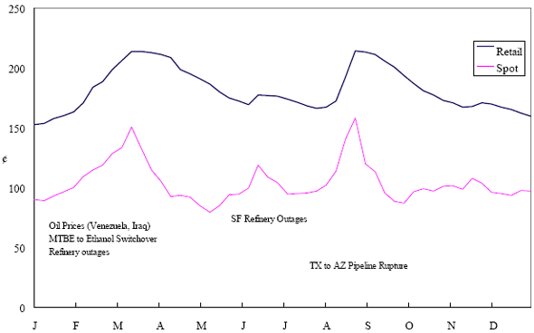
2003 Los Angeles Basin Gasoline Retail and Spot Prices
Figure 1: Plot of retail and wholesale spot prices for gasoline in Los Angeles.
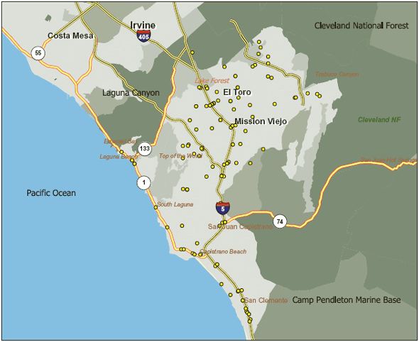
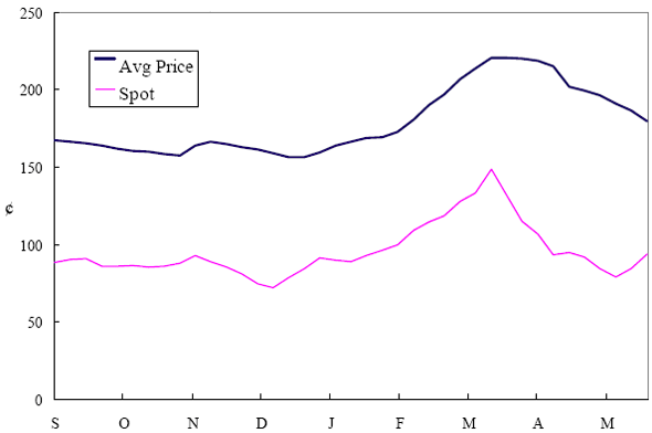
Figure 2: Map of South Orange County and Gasoline Stations. South Orange County Gasoline Retail and Spot Prices
Figure 3: Plot of retail and wholesale spot prices for gasoline in South Orange County.
Figure 4: Plotting the effect of a $1 cost shock. Panel a describes the path of cumulative price changes for both a postive and a negative cost shock (modified to the positive domain). Panel b describes the difference in these two effects.
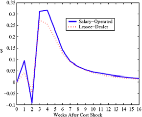
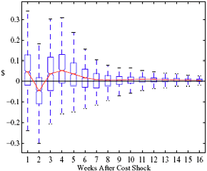
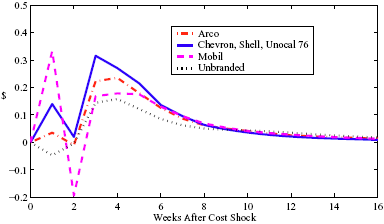
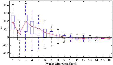
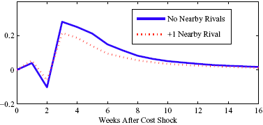
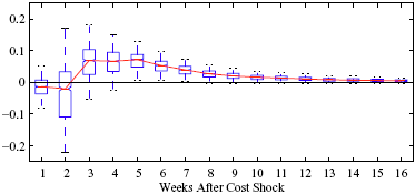
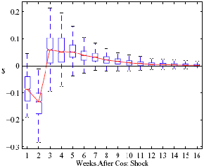
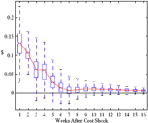
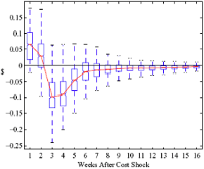
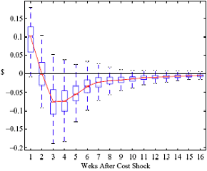
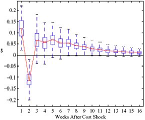
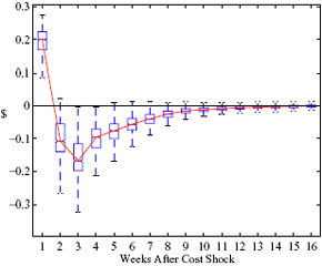
Figure 5: Charting the effect of a $1 cost shock for different organization types: Salary-operated versus lessee-dealer. Panel a describes the path of cumulative price changes for a salary-operated station. Panel b describes the path if these stations were switched to lessee-dealer. Panel c compares the difference in positive versus negative cost shocks for both types, and panel d describes the difference between the two effects from panel c. Asymmetry by Brand Identity Difference in Asymmetry: Branded minus Unbranded Figure 6: Charting the effect of brand identity on price response asymmetry. Panel a describes the difference in price responses for positive versus negative cost shocks across different brand types. Panel b plots the difference in asymmetries for branded versus un-branded stations. Marginal Effect of Nearby Competition on Asymmetry Difference in Asymmetry: Adding a Rival Station Nearby Figure 7: Charting the effect of rival proximity on price response asymmetry. Panel a describes the difference in price responses for positive versus negative cost shocks for stations with no immediate rivals and for stations with 1 rival added less than 0.1 miles away. Panel b plots the difference in these predictive asymmetries.
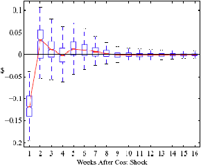
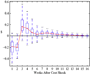
Figure 8: Charting the effects of site-level characteristics on price response asymmetry. Panels a and d describe the predictive change in price response asymmetry from increasing the observed characteristic for each station by one standard deviation. Panels b and c describe the predictive change for stations in having the observed characteristic versus removing it.
Figure 9: Charting the effects of local market-level characteristics on price response asymmetry. Panels a and b describe the predictive change in price response asymmetry for stations in having the observed characteristic versus removing it. Panels c and d describe the predictive change from increasing the observed characteristic for each station by one standard deviation. References Balke, Nathan S., Stephen P.A. Brown, and Mine K. Yücel, "Crude Oil and Gasoline Prices: An Asymmetric Relationship?" Federal Reserve Bank of Dallas Economic Review (First Quarter 1998). Banerjee, Sudipto, Bradley P. Carlin, and Alan E. Gelfand, "Hierarchical Modeling and Analysis for Spatial Data" Chapman & Hall, Boca Raton (2004). Barron, John M., John R. Umbeck, and Glen R. Waddell, "Consumer and Competitor Reactions: Evidence From a Retail-Gasoline Field Experiment" Working Paper, Department of Economics, Purdue University and Department of Economics, University of Oregon (September 2003). Bauwens, Luc, Michel Lubrano, and Jean-François Richard, "Bayesian Inference in Dynamic Econometric Models" Oxford University Press, Oxford (1999). Borenstein, Severin, "Selling Costs and Switching Costs: Explaining Retail Gasoline Margins," RAND Journal of Economics 22 (Autumn 1991), 354-369. Borenstein, Severin and Andrea Shepard, "Dynamic Pricing in Retail Gasoline Markets" RAND Journal of Economics 27 (1996), 429-451. Borenstein, Severin and Andrea Shepard, "Sticky Prices, Inventories, and Market Power in Wholesale Gasoline Markets" RAND Journal of Economics 33 (2002), 116-139. Borenstein, Severin, A. Colin Cameron, and Richard Gilbert, "Do Gasoline Prices Respond Asymmetrically to Crude Oil Price Changes?" Quarterly Journal of Economics 112 (February 1997), 305-339. Bulow, Jeremy I. and Paul Pfleiderer, "A Note on the Effect of Cost Changes on Prices," Journal of Political Economy 91 (February 1983), 182-185. Carlton, Dennis W. and Jeffrey M. Perloff, "Modern Industrial Organization" 4th Ed., Addison Wesley, Boston (2005). Chang, Myong-Hun, "The Effects of Product Differentiation on Collusive Pricing" International Journal of Industrial Organization 9 (1991), 453-469. Chang, Myong-Hun, "Intertemporal Product Choice and its Effects on Collusive Firm Behavior" International Economic Review 4 (1992), 773-793. Chib, Siddhartha and Bradley P. Carlin, "On MCMC Sampling in Hierarchical Longitudinal Models" Statistics and Computing 9 (1999), 17-26. Dahl, Carol and Thomas Sterner, "Analysing Gasoline Demand Elasticities: A Survey" Energy Economics 13 (1991), 203-210. Deltas, George, "Retail Gasoline Price Response Stickiness and Asymmetry to Wholesale Price Changes: The Effect of Local Market Power" Working Paper, Department of Economics, University of Illinois-Urbana Champaign (August 2004). Duffy-Deno, Kevin T., "Retail Price Asymmetries in Local Gasoline Markets" Energy Economics 18 (1996), 81-92. (EIA) Energy Information Administration "2003 Gasoline Price Study: Final Report" SR/O&G/2003-03 (November 2003). Engle, Robert F. and C. W.J. Granger, "Co-Integration and Error Correction: Representation, Estimation, and Testing" Econometrica 55 (March 1987), 251-276. Gupta, Barnali and Guhan Venkatu, "Tacit Collusion in a Spatial Model with Delivered Pricing" Journal of Economics 76 (2002), 49-64. Hackner, Jonas, "Endogenous product design in an infinitely repeated game" International Journal of Industrial Organization 13 (1995), 277-299. Hackner, Jonas, "Optimal Symmetric Punishments in a Bertrand Differentiated Products Duopoly" International Journal of Industrial Organization 14 (1996), 611-630. Haltiwanger, John. and Joseph E. Harrington Jr., "The Impact of Cyclical Demand Movements in Collusive Behavior" RAND Journal of Economics 22 (1991), 89-106. Hastings, Justine, "Vertical Relationships and Competition in Retail Gasoline Markets: An Empirical Evidence from Contract Changes in Southern California" Competition Policy Center Working Paper, Institute of Business and Economic Research, University of California, Berkeley (2000). Lewis, Matt, "Asymmetric Price Adjustment and Consumer Search: An Examination of the Retail Gasoline Market" Center for the Study of Energy Markets Working Paper, University of California Energy Institute, Berkeley (2003). Lindley, D.V. and A.F.M. Smith, "Bayes Estimates for the Linear Model (With Discussion)" Journal of the Royal Statistical Society B 34 (1972), 1-41. Manuszak, Mark D., "The Impact of Upstream Mergers on Retail Gasoline Markets" Working Paper, Graduate School of Industrial Administration, Carnegie Mellon University (December 2001). Poirier, Dale J., "Intermediate Statistics and Econometrics: A Comparative Approach" The MIT Press, Cambridge (1995). Rotemberg, Julio J. and Garth Saloner, "A Supergame-Theoretic Model of Price Wars during Booms" American Economic Review 76 (June 1986), 390-407. Romley, John A., "Demand Complementarity in Retail Markets: Measuring the Effects of Convenience Goods on the Demand for Gas" Ph.D. Dissertation, Stanford University (December 2002). Ross, Thomas W., "Cartel Stability and Product Differentiation" International Journal of Industrial Organization 10 (1992), 1-13. Shepard, Andrea, "Price Discrimination and Retail Configuration" Journal of Political Economy 99 (February 1991), 30-53. Slade, Margaret E., "Vancouver's Gasoline-Price Wars: An Empirical Exercise in Uncovering Supergame Strategies" Review of Economic Studies 59 (1992), 257-276. Stigler, George J., "A Theory of Oligopoly" Journal of Political Economy 72 (1964), 44-61. Tirole, Jean, "The Theory of Industrial Organization" The MIT Press, Cambridge (1988). Recent Economic Analysis Group Discussion Papers
Individual copies of papers are available free of charge from: Janet Ficco FOOTNOTES 12 See, for example, BCG, Balke et al. (1998), and Lewis (2003).
We then make the following substitutions: plug in
[D] and 16 This is the approach taken in BCG and Lewis(2003). 24 See the discussion that follows for a possible explanation for the Arco and Mobil difference. | |||||||||||||||||||||||||||||||||||||||||||||||||||||||||||||||||||||||||||||||||||||||||||||||||||||||||||||||||||||||||||||||||||||||||||||||||||||||||||||||||||||||||||||||||||||||||||||||||||||||||||||||||||||||||||||||||||||||||||||||||||||||||||||||||||||||||||||||||||||||||||||||||||||||||||||||||||||||||||||||||||||||||||||||||||||||||||||||||||||||||||||||||||||||||||||||||||||||||||||||||||||||||||||||||||||||||||||||||||||||||||||||||||||||||||||||||||||||||||||||||||||||||||||||||||||||||||||||||||||||||||||||||||||||||||||||||||||||||||||||||||||||||||||||||||||||||||||||||||||||||||||||||||||||||||||||||||||||||||||||||||||||||||||||||||||||||||||||||||||||||||||||||||||||||||||||||||||||||||||||||||||||||||||||||||||||||||||||||||||||||||||||||||||||||||||||||||||||||||||||||||||||||||||||||||||||||||||||||||||||||||||||||||||||||||||||||||||||||||||||||||||||||||||||||||||||||||||||||||||||||||||||||||||||||||||||||||||||||||||||||||||||||||||||||||||||||||||||||||||||

 U.S. Department
of Justice
 is such that
  and perfect collusion (monopoly pricing) is assured when
  , where
  denotes the discount factor above which monopoly pricing is the best achievable collusive price where no firm has an incentive to deviate. This relationship implies that collusion is easier to sustain the fewer the number of firms there are in the market. To derive a prediction on what happens to price-response asymmetry when the number of firms changes, I focus on what happens when
  . In the HH model, the only sustainable collusive price path when
  . Provided there is continuity, price-response asymmetry will be increasing in
  ). Since
  is increasing in n, it follows that the range of asymmetry-inducing
 , so that ct = ct-1 ... = ct-j-1 =

 . When combined with the derivative of (2) with respect to
  , then, conditional on some value for
  and
and  .
.  is exactly equal to the long-run expected markup.
  pst = pst - ps,t-1 and
 ,
,  and
and  are specific to the number of initial price and costs lags in the levels specification.
  , can be thought of as the (one period lagged) deviation in prices from their long-run expected relationship with costs, which means that
  is the short-run correction in current prices that helps bring retail prices back to their equilibrium relationship with costs. When prices exceed costs by more than the long-run markup, we would expect downward pressure on current prices until the long-run markup is restored, and thus I expect
  and substitute these residuals in place of the error correction term in a least squares regression of (3) .
 with certainty, analogous to the final approach taken in Lewis (2003) after the one-step procedure there revealed an estimated
  .
.  denote the indicator function, which takes on the value 1 when the interior condition
  is met, a parsimonious representation of response asymmetry is
 , while for a positive cost shock, the contribution is
  .
.  and ct = 0 (so that prices are currently at their long-run equilibrium), and then let
  . At t + 2, the cumulative price change is

 to
to  . Lastly, I define an asymmetry function,
  , as the difference between the positive and negative CRFs, i.e.,
 ), and that station-level markups are fixed constants. After establishing this basic asymmetry, I then explore the data further by introducing random effects for each of the coefficients and interact them with the observed station-varying characteristics in my data. The random coefficients model is explained in more detail later.
  with standard error 0.29 in that study), despite having 92 weekly observations compared to my 39. On balance, it would appear that the data strongly favor
  > 1, especially in light of the of the data significantly updating my highly informative prior specification.
  , where for a firm that faces imperfect substitutes the elasticity
  is less than -1. While I would stress that this is a highly stylized assumption, if indeed the stations in my dataset face constant elasticty residual demand, the implied average station-level elasticity when
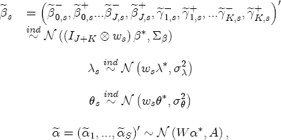
 , associated now with the covariate vector xst(
 ). Under these assumptions, the model is now described as a hierarchical error correction model (H-ECM) that centers each covariate in (4) at a linear combination of the L observed station-level characteristics in the vector ws. Hence,
  is the (J + K) L vector of coefficients in the second-stage analysis. Alternatively, if we integrate over the distributional assumption on
  ,
,  , and
, and  are the L vectors of coefficients for the remaining parameters.
 parameters on the characteristics described in Table 2. To interpret this summary output, recall that we expect
  is eased by formation of a matrix composed of a constant, S - 1 station dummies, and the vector of one-period lagged costs for each station. Thus
  is the markup for the excluded station, which I describe with a normal density, centered at 0.8 with a variance of 5; the remaining S - 1 station dummy coefficients are centered at 0, also with a variance of 5. I interpret this prior information as being highly diffuse, centered at reasonable a priori values. Diffuseness, however, is an inappropriate specification for the long-run price response to costs represented in
  and
and  , I revert to diffuseness with cues taken from BCG. I condition the analysis on J = 3 and K = 2, which results in 3 cost-difference regressors and 2 price-difference regressors. My prior on
  ,
,  and
and  is such that negative changes are centered at 0, while positive changes are centered at 0.1, reflecting an a priori expectation of a positive asymmetry difference. Uncertainty about the appropriateness of the additional lags leads me to center all of the coefficients in
  and
and  at zero. For all of the short-run changes in cost and price coefficients, the variance is set at 5, which again represents a diffuse specification that highly favors the likelihood information over the prior. For the short-run response to the deviation from equilibrium,
  ), and thus require a prior specification for the residual variance term in addition to the coefficients described above. Recall the usual specification for goodness of fit, R2 = 1 - SSE/SST, where SSE is the sum of squared errors and SST is the total sum of squares. Also recall the classical estimator for
  , the minimum integer value that v can be to ensure a prior mean is 3, which is the value I use in this study. Specifically, I center my prior information on the residual variance near the implied value for s2 that results from R2 = 0.25 and SST the actual variance in the data times the sample size. But since v = 3, this results in a prior distribution that, like those for the coefficients above, is highly diffuse. Indeed, it places so much weight in the tails of the distribution that the prior variance of
  ,
,  ,
,  ,
,  and
and  . Then, for m = 1, ..., M:
  ,
,  ,
,  ,
,  ,
,  ,
, 
 ,
,  ,
,  ,
,  ,
,  ,
,  ,
,  ,
,  and
and  denote an arbitrary coefficient in the first-stage regression (e.g.,
  or
or  ). Recall the distributional assumption on these coefficients that the marginal density for one of the coefficients is
  . In the original setup with
  , when
  was
was  ,
,  or
or  , I centered the prior at zero, while for the associated positive effects the prior was centered at 0.1. I maintain that specification through the prior on
  . Since ws contains a constant plus a set of station-level covariates, about which I want the data to be the primary source of information, I center
  , where
  has elements as just described above and In is the identity matrix of size n. Additionally, since I do not want to a priori enforce large heterogeneity in responses, I set
  at 0.01. In the stacked vector
  at 0.01I(j+k). Under an inverse Wishart prior for
  , with
  as just described. Again, I do not want to introduce heterogeneity in the
  , with centrality parameter s2 set at 0.01 and v = 3 to emphasize diffuseness.
  to be 1 and the remaining coefficients at 0, and then place a prior variance on each element of
  of 0.1/6, similar to the prior for the basic model. The prior information on
  is identical to that for
  .
.  . These parameters must remain in the positive domain to ensure a stable and positive definite covariance matrix A. For this reason, I work with the reparameterized vector
  , about which I assume a normal prior centered at log (0.1, 0.1, 0.01) with prior covariance matrix I3. With
  centered at 0.01, there is a strong a priori belief that the correlation in markups between stations depends inversely on the distance between them, although with the prior information on
  and
and  , because of the near-conjugacy of my prior this is a trivial extension to the basic Gibbs sampler. The only complication for


 denotes a Ts vector of ones. Further letting
  , we obtain the full vector of stacked observations (first over time, then over station)
 and let
  and
and  equal the vector of sample averages over time of ys for each station. Then following Lindley and Smith (1972), we have that
  ,
,  ,
,  , where


 and
and  are discussed in Section A.3 above.
  of 0.0039 with a posterior standard deviation of 0.003. Together with the other parameters in
  . In Table A2, I summarize the predicted marginal effects of each of the station characteristics on the estimated markup of retail over wholesale spot prices when the spot price is $1.
 )
)


 , the expected value of demand. Since demand is iid, the following period's expectation of demand is
 for
for  on the left, and on the right substitute
  for
for  for
for  for
for  for
for  for
for  for
for  . With these substitions, we get

 .
.  , the parameters in the error correction term (
 . Bauwens et al. (1999) propose a joint prior between
  , as a practical matter the markups in my data set appear to be highly positively correlated.
  , which clearly depends on the price data. But the elicitation itself is very intuitive. It amounts to a prior expectation for both R2 and the underlying variance in the data. The difficulty comes in that the data variance is a basic descriptive statistic that the researcher will always know before estimation of the model, and which is information he cannot forget when constructing prior beliefs about the model's fit. In a practical sense, this procedure results in centering the prior for